Examples¶

Basic Example - Residential Price Hedonic¶

A fairly complete case study of using UrbanSim can be shown entirely within a single Jupyter Notebook, as is the case with this Notebook from the example repository.

As the canonical example of using UrbanSim, take the case of a residential sales hedonic model used to perform an ordinary least squares regression on a table of building price data. The best practice would be to store the building data in a Pandas HDFStore, and the buildings table can include millions of rows (all of the buildings in a region) and attributes like square footage, lot size, number of bedrooms and bathrooms and the like. Importantly, the dependent variable should also be included which in this case might be the assessed or observed price of each unit. The example repository includes sample data so that this Notebook can be executed.

This Notebook performs the exact same residential price hedonic as in the complete example below, but all entirely within the same Jupyter Notebook (and without explicitly using the @orca.step decorator). The simplest use case of the UrbanSim methodology is to create a single model to study an empirical behavior of interest to the modeler, and a good place to start in building such a model is this example.

Note that the flow of the notebook is one often followed in statistical modeling:

Import the necessary modules
Set the data repository (HDFStore)
Name the actual tables from the repository (and set a relationship between zones and buildings)
Set all columns which are computed from the source data - for instance, map specific building_type_ids to a general_type column or sum the number of residential units in a zone using the sum_residential_units variable and so forth. Note that the vast majority of code in this notebook is in creating computed columns
Next instantiate and configure the RegressionModel instance for the hedonic, including some filters which get rid of degenerate data
Then merge the buildings and zones tables and fill invalid numeric values with reasonable imputations (medians, modes, or zeros respectively)
Then fit the model and print the fit summary
And finally run the model in predict mode and describe the predicted values

If you can follow this simple functionality, most of UrbanSim simply repeats this sort of flow for other urban behaviors. It’s probably a good idea to read through this example a few times until it’s relatively clear how the parts fit together before moving on to the complete example. For the complete example, a process like the one described above is then repeated for each model of urban behavior described in the gentle introduction to UrbanSim.

Note that there is often some overlap in data needs for different models - for instance, both the residential and non-residential hedonic models in the implementation below use the same buildings table to compute the relevant variables (although the variables that are utilized are often slightly different). Thus it is usually good practice to abstract bits of functionality into different parts of the model system to aid in code reuse. A full example follows which shows exactly how this can be done.

Complete Example - San Francisco UrbanSim Modules¶

A complete example of the latest UrbanSim framework is now being maintained on GitHub. The example requires that the UrbanSim package is already installed (no other dependencies are required). The example is maintained under Travis Continuous Integration so should always run with the latest version of UrbanSim.

The example has a number of Python modules including dataset.py, assumptions.py, variables.py, models.py which will be discussed one at a time below. The modules are then used in workflows which are Jupyter Notebooks and will be described in detail in the following section.

Table Sources¶

Data can be loaded into the simulation framework using the Orca table decorator with functions that describe where the data comes from. Registered tables return Pandas DataFrames but the data can come from different locations, including HDF5 files, CSV files, databases, Excel files, and others. Pandas has a large and ever-expanding set of data connectivity modules although this example keeps data in a single HDF5 data store which is provided directly in the repo.

Specifying a source of data for a DataFrame is done with the orca.table decorator as in the code below, which is lifted directly from the example.

@orca.table('households')
def households(store):
    df = store['households']
    return df

The complete example includes mappings of tables stored in the HDF5 file to table sources for a typical UrbanSim schema, including parcels, buildings, households, jobs, zoning (density limits and allowable uses), and zones (aggregate geographic shapes in the city). By convention these table sources are stored in the dataset.py file but this is not a strict requirement.

Arbitrary Python can occur in these table sources as shown in the zoning_baseline table source which uses injections of zoning and zoning_for_parcels that were defined in the prior lines of code.

Finally, the relationships between all tables can be specified with the orca.broadcast() function and all of the broadcasts for the example are specified together at the bottom of the dataset.py file. Once these relationships are set they can be used later in the simulation using the merge_tables function.

Assumptions¶

By convention assumptions.py contains all of the high-level assumptions for the simulation. A typical assumption would be the one below, which sets a Python dictionary that can be used to map building types to land use category names.

# this maps building type ids to general building types
# basically just reduces dimensionality
sim.add_injectable("building_type_map", {
"Residential",
"Residential",
"Residential",
"Office",
"Hotel",
"School",
"Industrial",
"Industrial",
"Industrial",
"Retail",
"Retail",
"Residential",
"Retail",
"Office"
})

In this example, all assumptions are registered using the orca.add_injectable method, which is used to register Python data types with names that can be injected to other Orca methods. Like Orca tables and columns, injectables can also be added using the orca.injectable decorator as well. Although not all injectables are assumptions, this file mostly contains high-level assumptions including a dictionary of building square feet per job for each building type, a map of building forms to building types, etc.

Note that the above code simply sets the map to the name building_type_map - it must be injected and used somewhere else to have an effect. In fact, this map is used in variables.py to compute the general_type attribute on the buildings table.

Perhaps most importantly, the location of the HDFStore is set using the store injectable. An observant reader will notice that this store injectable which is set here was used in the table_source described above. Note that the store injectable could be defined after the households table_source as long as they’re both registered before the simulation makes an attempt to call the registered methods.

Variables¶

variables.py is similar to the variable library from the OPUS version of UrbanSim. By convention all variables which are computed from underlying attributes are stored in this file. Although the previous version of UrbanSim used a domain-specific expression language, the current version uses native Pandas, along with the @orca.column decorator and dependency injection. As before, the convention is to name the underlying data the primary attributes and the functions specified here as computed columns. A typical example is shown below:

@orca.column('zones', 'sum_residential_units')
def sum_residential_units(buildings):
    return buildings.residential_units.groupby(buildings.zone_id).sum()

This creates a new column sum_residential_units for the zones table. Notice that because of the magic of groupby, the grouping column is used as the index after the operation so although buildings has been passed in here, because zone_id is available on the buildings table, the Series that is returned is appropriate as a column on the zones table. In other words groupby is used to aggregate from the buildings table to the zones table, which is a very common operation.

To move an attribute from one table to another using a foreign key, the misc module has a reindex method. Thus even though zone_id is only a primary attribute on the parcels table, it can be moved using reindex to the buildings table using the parcel_id (foreign key) of that table. This is shown below and extracted from the example.

@orca.column('buildings', 'zone_id', cache=True)
def zone_id(buildings, parcels):
    return misc.reindex(parcels.zone_id, buildings.parcel_id)

Note that computed columns can also be used in other computed columns. For instance buildings.zone_id in the code for the sum_residential_units columns is itself a computed column (defined by the code we just saw).

This is the real power of the framework. The decorators define a hierarchy of dependent columns, which are dependent on other dependent columns, which are themselves dependent on primary attributes, which are likely dependent on injectables and table_sources. In fact, the models we see next are usually what actually resolves these dependencies, and no variables are computed unless they are actually required by the models. The user is relatively agnostic to this whole process and need only define a line or two of code at a time attached to the proper data concept. Thus a whole data processing workflow can be built from the hierarchy of concepts within the simulation framework.

A Note on Table Wrappers

The buildings object that gets passed in is a DataFrame Wrapper and the reader is referred to the API documentation to learn more about this concept. In general, this means the user has access to the Series object by name on the wrapper but the full set of Pandas DataFrame methods is not necessarily available. For instance .loc and .groupby will both yield exceptions on the DataFrameWrapper.

To convert a DataFrameWrapper to a DataFrame, the user can simply call to_frame but this returns all computed columns on the table and so has performance implications. In general it’s better to use the Series objects directly where possible.

As a concrete example, the following code is recommended:

return buildings.residential_units.groupby(buildings.zone_id).sum()

This will not work:

return buildings.groupby("zone_id").residential_units.sum()

This will work but is slow.

return buildings.to_frame().groupby("zone_id").residential_units.sum()

One workaround is to call to_frame with only the columns you need, although this is a verbose syntax, i.e. this will work but is syntactically awkward.

return buildings.to_frame(['zone_id', 'residential_units']).groupby("zone_id").residential_units.sum()

Finally, if all the attributes being used are primary, the user can call local_columns without serious performance degradation.

return buildings.to_frame(buildings.local_columns).groupby("zone_id").residential_units.sum()

Models¶

The main objective of the models.py file is to define the “entry points” into the model system. Although UrbanSim provides the direct API for a Regression Model, a Location Choice Model, etc, it is the models.py file which defines the specific steps that outline a simulation or even a more general data processing workflow.

In the San Francisco example, there are two price/rent hedonic models which both use the RegressionModel, one which is the residential sales hedonic which is estimated with the entry point rsh_estimate and then run in simulation mode with the entry point rsh_simulate. The non-residential rent hedonic has similar entry points nrh_estimate and nrh_simulate. Note that both functions call hedonic_estimate and hedonic_simulate in utils.py. In this case utils.py actually uses the UrbanSim API by calling the fit_from_cfg method on the Regressionmodel.

There are two things that warrant further explanation at this point.

utils.py is a set of helper functions that assist with merging data and running models from configuration files. Note that the code in this file is generally shareable across UrbanSim implementations (in fact, this exact code is in use in multiple live simulations). It defines a certain style of UrbanSim and handles a number of boundary cases in a transparent way. In the long run, this kind of functionality might be unit tested and moved to UrbanSim, but for now we think it helps with transparency, flexibility, and debugging to keep this file with the specific client implementations.
Many of the models use configuration files to define the actual model configuration. In fact, most models in this file are very short stub functions which pass a Pandas DataFrame into the estimation and configure the model using a configuration file in the YAML file format. For instance, the rsh_estimate function knows to read the configuration file, estimate the model defined in the configuration on the dataframe passed in, and write the estimated coefficients back to the same configuration file, and the complete method is pasted below:
```
@orca.step('rsh_estimate')
def rsh_estimate(buildings, zones):
    return utils.hedonic_estimate("rsh.yaml", buildings, zones)
```

For simulation, the stub is only slightly more complicated - in this case the model is simulating an output based on the model we estimated above, and the resulting Pandas Series needs to be stored on an UrbanSim table with a given attribute name (in this case to the residential_sales_price attribute of buildings table).:
@orca.step('rsh_simulate')
def rsh_simulate(buildings, zones):
    return utils.hedonic_simulate("rsh.yaml", buildings, zones,
                              "residential_sales_price")

These stubs can then be repeated as necessary with quite a bit of flexibility. For instance, the live Bay Area UrbanSim implementation has an additional hedonic model for residential rent which is not present in the example, and the associated stubs make use of a new configuration file called rrh.yaml and so forth.

A typical UrbanSim models setup is present in the models.py file, which registers 15 models including hedonic models, location choice models, relocation models, and transition models for both the residential and non-residential sides of the real estate market, then a feasibility model which uses the prices simulated previously to measure real estate development feasibility, and a developer model for each of the residential and non-residential sides.

Note that some parameters are defined directly in Python while other models have full configuration files to specify the model configuration. This is a matter of taste, and eventually all of the models are likely to be YAML configurable.

Note also that some models have dependencies on previous models. For instance hlcm_simulate and feasibility are both dependent on rsh_simulate. At this time there is no way to guarantee that model dependencies are met and this is left to the user to resolve. For full simulations, there is a typical order of models which doesn’t change very often, so this requirement is not terribly onerous.

Clearly models.py is extremely flexible - any method which reads and writes data using the simulation framework can be considered a model. Models with more logic than the stubs above are common, although more complicated functionality should eventually be generalized, documented, unit tested, and added to UrbanSim. In the future new travel modeling and data cleaning workflows will be implemented in the same framework.

One final point about models.py - these entry points are designed to be written by the model implementer and not necessarily the modeler herself. Once the models have been correctly set up, the basic infrastructure of the model will rarely change. What happens more frequently is 1) a new data source is added 2) a new variable is computed with a column from that data source and then 3) that variable is added to the YAML configuration for one of the statistical models. The framework is designed to enable these changes, and because of this models.py is the least frequent to change of the modules described here. models.py defines the structure of the simulation while the other modules enable the configuration.

Model Configuration¶

Bridging the divide between the modules above and the workflows below are the configuration files. Note that models can be configured directly in Python code (as in the basic example) or in YAML configuration files (as in the complete example). If using the utils.py methods above, the simulation is set up to read and write from the configuration files.

The example has four configuration files which can be navigated on the GitHub site. The rsh.yaml file has a mixture of input and output parameters and the complete set of input parameters is displayed below.

name: rsh

model_type: regression

fit_filters:
- unit_lot_size > 0
- year_built > 1000
- year_built < 2020
- unit_sqft > 100
- unit_sqft < 20000

predict_filters:
- general_type == 'Residential'

model_expression: np.log1p(residential_sales_price) ~ I(year_built < 1940) + I(year_built
    > 2005) + np.log1p(unit_sqft) + np.log1p(unit_lot_size) + sum_residential_units
    + ave_lot_sqft + ave_unit_sqft + ave_income

ytransform: np.exp

Notice that the parameters name, fit_filters, predict_filters, model_expression, and y_transform are the exact same parameters provided to the RegressionModel object in the api. This is by design, so that the API documentation also documents the configuration files although an example configuration is a great place to get started while using the API pages as a reference.

YAML configuration files currently can also be used to define location choice models and even accessibility variables, and in theory can be added to any UrbanSim model that supports YAML persistence as described in the API docs. Using configuration files specified in YAML also allows interactivity with the UrbanSim web portal, which is one of the main reasons for following this architecture.

As can be seen, these configuration files are a great way to separate specification of the model from the actual infrastructure that stores and uses these configuration files and the data which gets passed to the models, both of which are defined in the models.py file. As stated before, models.py entry points define the structure of the simulation while the YAML files are used to configure the models.

Complete Example - San Francisco UrbanSim Workflows¶

Once the proper setup of Python modules is accomplished as above, interactive execution of certain UrbanSim workflows is extremely easy to accomplish, and will be described in the subsections below. These are all done in the Jupyter Notebook and use nbviewer to display the results in a web browser. We use Jupyter Notebooks (or the UrbanSim web portal) for almost any workflow in order to avoid executing Python from the command line / console, although this is an option as well.

Note that because these workflows are Jupyter Notebooks, the reader should browse to the example on the web and no example code will be pasted here.

One thing to note is the autoreload magic used in all of these workflows. This can be very helpful when interactively editing code in the underlying Python modules as it automatically keeps the code in sync within the notebooks (i.e. it re-imports the modules when the underlying code changes).

Estimation Workflow¶

A sample estimation workflow is available in this Notebook.

This notebook estimates all of the models in the example that need estimation (because they are statistical models). In fact, every cell simply calls the orca.run method with one of the names of the model entry points defined in models.py. The orca.run method resolves all of the dependencies and prints the output of the model estimation in the result cell of the Jupyter Notebook. Note that the hedonic models are estimated first, then simulated, and then the location choice models are estimated since the hedonic models are dependencies of the location choice models. In other words, the rsh_simulate method is configured to create the residential_sales_price column which is then a right hand side variable in the hlcm_estimate model (because residential price is theorized to impact the location choices of households).

Simulation Workflow¶

A sample simulation workflow (a complete UrbanSim simulation) is available in this Notebook.

This notebook is possibly even simpler than the estimation workflow as it has only one substantive cell which runs all of the available models in the appropriate sequence. Passing a range of years will run the simulation for multiple years (the example simply runs the simulation for a single year). Other parameters are available to the orca.run method which write the output to an HDF5 file.

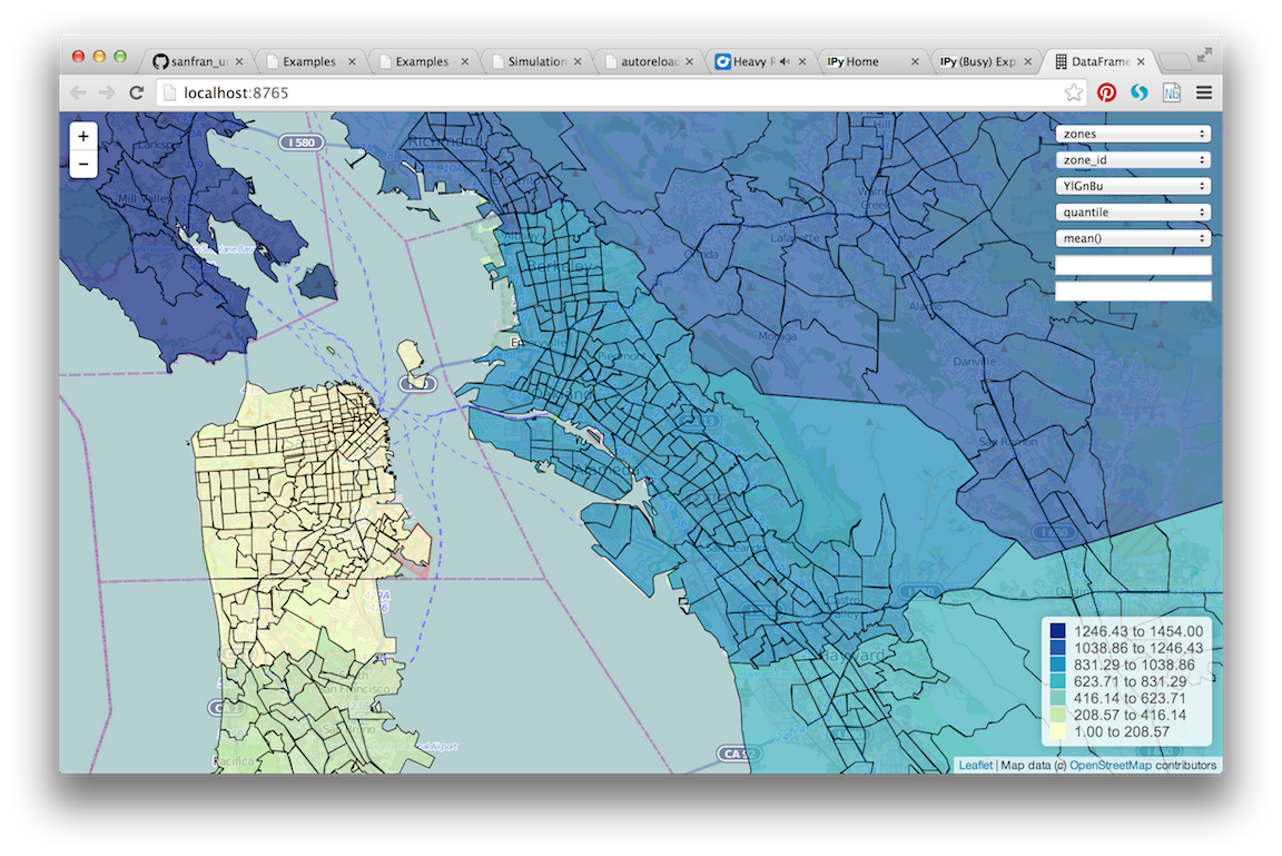
Exploration Workflow¶

UrbanSim now also provides a method to interactively explore UrbanSim inputs and outputs using web mapping tools, and the exploration notebook demonstrates how to set up and use this interactive display tool.

This is another simple and powerful notebook which can be used to quickly map variables of both base year and simulated data without leaving the workflow to use GIS tools. This example first creates the DataFrames for many of the UrbanSim tables that have been registered (buildings, househlds, jobs, and others). Once the DataFrames have been created, they are passed to the start method.

See DataFrame Explorer for detailed information on how to call the start method and what queries the website is performing.

Once the start method has been called, the Jupyter Notebook is running a web service which will respond to queries from a web browser. Try it out - open your web browser and navigate to http://localhost:8765/ or follow the same link embedded in your notebook. Note the link won’t work on the web example - you need to have the example running on your local machine - all queries are run interactively between your web browser and the Jupyter Notebook. Your web browser should show a page like the following:

See Website Description for a description of how to use the website that is rendered.

Because the web service is serving these queries directly from the Jupyter Notebook, you can execute some part of a data processing workflow, then run dframe_explorer and look at the results. If something needs modification, simply hit the interrupt kernel menu item in the Jupyter Notebook. You can now execute more Notebook cells and return to dframe_explorer at any time by running the appropriate cell again. Now map exploration is simply another interactive step in your data processing workflow.

Model Implementation Choices¶

There are a number of model implementation choices that can be made in implementing an UrbanSim regional forecasting tool, and this will describe a few of the possibilities. There is definitely a set of best practices though, so shoot us an email if you want more detail.

Geographic Detail¶

Although zone or block-level models can be done (and gridcells have been used historically), at this point the geographic detail is typically at the parcel or building level. If good information is available for individual units, this level or detail is actually ideal.

Most household and employment location choices choose building_ids at this point, and the number of available units is measured as the supply of units / job_spaces in the building minus the number of households / jobs in the building.

UrbanAccess or Zones¶

It is fairly standard to combine the buildings from the locations discussed above with some measure of the neighborhood around each building. The simplest implementation of this idea is used in the sanfran_example - and is typical of traditional GIS - which is to use aggregations within some higher level polygon. In the most common case, the region has zones assigned and every parcel is assigned a zone_id (the zone_id is then available on the other related tables). Once zone_ids are available, vanilla Pandas is usable and GIS is not strictly required.

Although this is the easiest implementation method, a pedestrian-scale network-based method is perhaps more appropriate when analyses are happening at the parcel- and building-scale and this is the exactly the intended purpose of the Pandana framework. Most full UrbanSim implementations now use aggregations along the local street network.

Jobs or Establishments¶

Jobs by sector is often the unit of analysis for the non-residential side, as this kind of model is completely analagous to the residential side and is perhaps the easiest to understand. In some cases establishments can be used instead of jobs to capture different behavior of different size establishments, but fitting establishments into buildings then becomes a tricky endeavor (and modeling the movements of large employers should not really be part of the scope of the model system).

Configuration of Models¶

Some choices need to made on the configuration of models. For instance, is there a single hedonic for residential sales price or is there a second model for rent? Is non-residential rent segmented by building type? How many different uses are there in the pro forma and what forms (mixes of uses) will be tested. The simplest model configuration is shown in the sanfran_urbansim example, and additional behavior can be captured to answer specific research questions.

Dealing with NaNs¶

There is not a standard method for dealing with NaNs (typically indicating missing data) within UrbanSim, but there is a good convention that can be used. First an injectable can be set with an object in this form (make sure to set the name appropriately):

orca.add_injectable("fillna_config", {
    "buildings": {
        "residential_sales_price": ("zero", "int"),
        "non_residential_rent": ("zero", "int"),
        "residential_units": ("zero", "int"),
        "non_residential_sqft": ("zero", "int"),
        "year_built": ("median", "int"),
        "building_type_id": ("mode", "int")
    },
    "jobs": {
        "job_category": ("mode", "str"),
    }
})

The keys in this object are table names, the values are also a dictionary where the keys are column names and the values are a tuple. The first value of the tuple is what to call the Pandas fillna function with, and can be a choice of “zero,” “median,” or “mode” and should be set appropriately by the user for the specific column. The second argument is the data type to convert to. The user can then call utils.fill_na_from_config as in the example with a DataFrame and table name and all NaNs will be filled. This functionality will eventually be moved into UrbanSim.