Tutorial
Note
This tutorial was last updated in 2017 and may not be current. The best place to start is with the Pandana demo notebook.
At this point it is probably helpful to make concrete the topics discussed in
the introduction by giving code sample. There is also an IPython Notebook
in the Pandana repo which gives the entire workflow,
but the discussion here will take things line-by-line with a sufficient
summary of the functionality.
Note that these code samples assume you have imported pandas and pandana as follows:
import pandas as pd
import pandana as pdna
Create the network
First create the network. Although the API is incredibly simple,
this is likely to be the most difficult part of using Pandana. In the future
we will leverage the import functionality of tools like geopandas to
directly access networks via shapefiles,
but for now the initialization pandana.network.Network.__init__()
takes a small number of Pandas Series objects.
The network is comprised of a set of nodes and edges. We store our nodes and edges as two Pandas DataFrames in an HDFStore object. We can access them as follows (the demo data file can be downloaded here):
store = pd.HDFStore('data/osm_bayarea.h5', "r")
nodes = store.nodes
edges = store.edges
print nodes.head(3)
print edges.head(3)
The output of the above code shows:
              x           y
8   629310.1250  4095536.75
9   629120.9375  4095816.75
10  628951.5625  4096090.50

[3 rows x 2 columns]

   from  to      weight
6     8   9  338.255005
7     9  10  322.532990
8    10  11  218.505997

[3 rows x 3 columns]
The data structure is very simple indeed. Nodes have an index which is the
id of the node and an x-y position. Much like shapely, Pandana is
agnostic to the coordinate system. Use your local coordinate system or
longitude then latitude - either one will work. Edges are then ids (which
aren’t used) and
from node ids and to node_ids which should index directly to the node
DataFrame. A weight column (or multiple weight columns) is (are) required
as the impedance for the network. Here, distance is used from OpenStreetMap
edges.
To create the network given the above DataFrames, simply call:
net=pdna.Network(nodes["x"], nodes["y"], edges["from"], edges["to"],
                 edges[["weight"]])
It’s probably a good idea (though not strictly required) to precompute a given horizon distance so that aggregations don’t perform the network queries unnecessarily. This is done by calling the following code, where 3000 meters is used as the horizon distance:
net.precompute(3000)
Note that a large amount of time is spent in the precomputations that take place for these two lines of code. On a MacBook, these two lines of code take 4 seconds and 8.5 seconds respectively.
This was done on a 4-core cpu, so if your precomputation is much slower,
check the IPython Notebook output (on the console) for a statement that says
Generating contraction hierarchies with 4 threads. If your output says
1 instead of 4 you are running single threaded. If you are running on
a multi-core cpu, there is probably a way to speed up the computation.
Nearest queries
Now for the fun part. Nearest queries are slightly easier, so let’s cover that first.
First initialize the POI (point-of-interest) category:
net.set_pois("restaurants", 2000, 10, x, y)
This code initializes the “restaurants” category with the positions specified by the x and y columns (which are Pandas Series), at a max distance of 2000 meters for up to the 10 nearest points-of-interest. Next perform the query:
Here is a link to the docs: pandana.network.Network.set_pois()
net.nearest_pois(2000, "restaurants", num_pois=10)
This searches for the 10 nearest restaurants and is exactly the query that is displayed in the introduction. This returns a DataFrame with the number of columns equal to the number of POIs that are requested. For instance, a describe of the output DataFrame look like this (note that the query executed in half a second:
CPU times: user 1.37 s, sys: 11 ms, total: 1.38 s
Wall time: 498 ms
                  1              2              3              4   \
count  226060.000000  226060.000000  226060.000000  226060.000000
mean     1542.487481    1676.578324    1746.392002    1794.982571
std       629.581983     543.853257     485.754919     440.356407
min         0.000000       0.000000       0.000000       0.000000
25%      1063.236542    1473.924011    1775.853271    2000.000000
50%      2000.000000    2000.000000    2000.000000    2000.000000
75%      2000.000000    2000.000000    2000.000000    2000.000000
max      2000.000000    2000.000000    2000.000000    2000.000000

                  5              6              7              8   \
count  226060.000000  226060.000000  226060.000000  226060.000000
mean     1825.214545    1846.061683    1864.423958    1879.123914
std       407.388660     380.878320     353.350067     330.835422
min         0.000000       0.000000       0.000000       0.000000
25%      2000.000000    2000.000000    2000.000000    2000.000000
50%      2000.000000    2000.000000    2000.000000    2000.000000
75%      2000.000000    2000.000000    2000.000000    2000.000000
max      2000.000000    2000.000000    2000.000000    2000.000000

                  9              10
count  226060.000000  226060.000000
mean     1893.909935    1908.403787
std       306.340819     283.554353
min         0.000000      56.143002
25%      2000.000000    2000.000000
50%      2000.000000    2000.000000
75%      2000.000000    2000.000000
max      2000.000000    2000.000000

[8 rows x 10 columns]
Here is a link to the docs: pandana.network.Network.nearest_pois()
Aggregation queries
Performing a general network aggregation isn’t much harder. In this case, it is assumed that DataFrames are much larger and that queries have a lot more variety.
For this reason, the workflow is typically to map the variables x and y to
node_ids (which can then be cached or written to disk at a later date) and
to call set for each data column, potentially several times. For instance,
if you have a DataFrame of buildings with x and y coordinates,
you can use get_node_ids to set node_ids as an attribute on the
buildings table and then set can be called many times with all the
attributes of the buildings table and their associated column names.
x, y = buildings.x, buildings.y
buildings["node_ids"] = net.get_node_ids(x, y)
net.set(node_ids, variable=buildings.square_footage, name="square_footage")
net.set(node_ids, variable=buildings.residential_units,
        name="residential_units")
Here is a link to the docs: pandana.network.Network.get_node_ids()
and pandana.network.Network.set()
Once the variables have been assigned to the network, the user can query the network repeatedly with different parameters.
s = net.aggregate(500, type="sum", decay="linear", name="square_footage")
t = net.aggregate(1000, type="sum", decay="linear", name="square_footage")
u = net.aggregate(2000, type="sum", decay="linear", name="square_footage")
v = net.aggregate(3000, type="sum", decay="linear", name="square_footage")
w = net.aggregate(3000, type="ave", decay="flat",
                  name="residential_units")
Here is a link to the docs: pandana.network.Network.aggregate()
Note that if networks have been indexed and precomputed, the aggregations should take less than a second up to a distance of roughly three kilometers for a network with a few hundred thousand nodes.
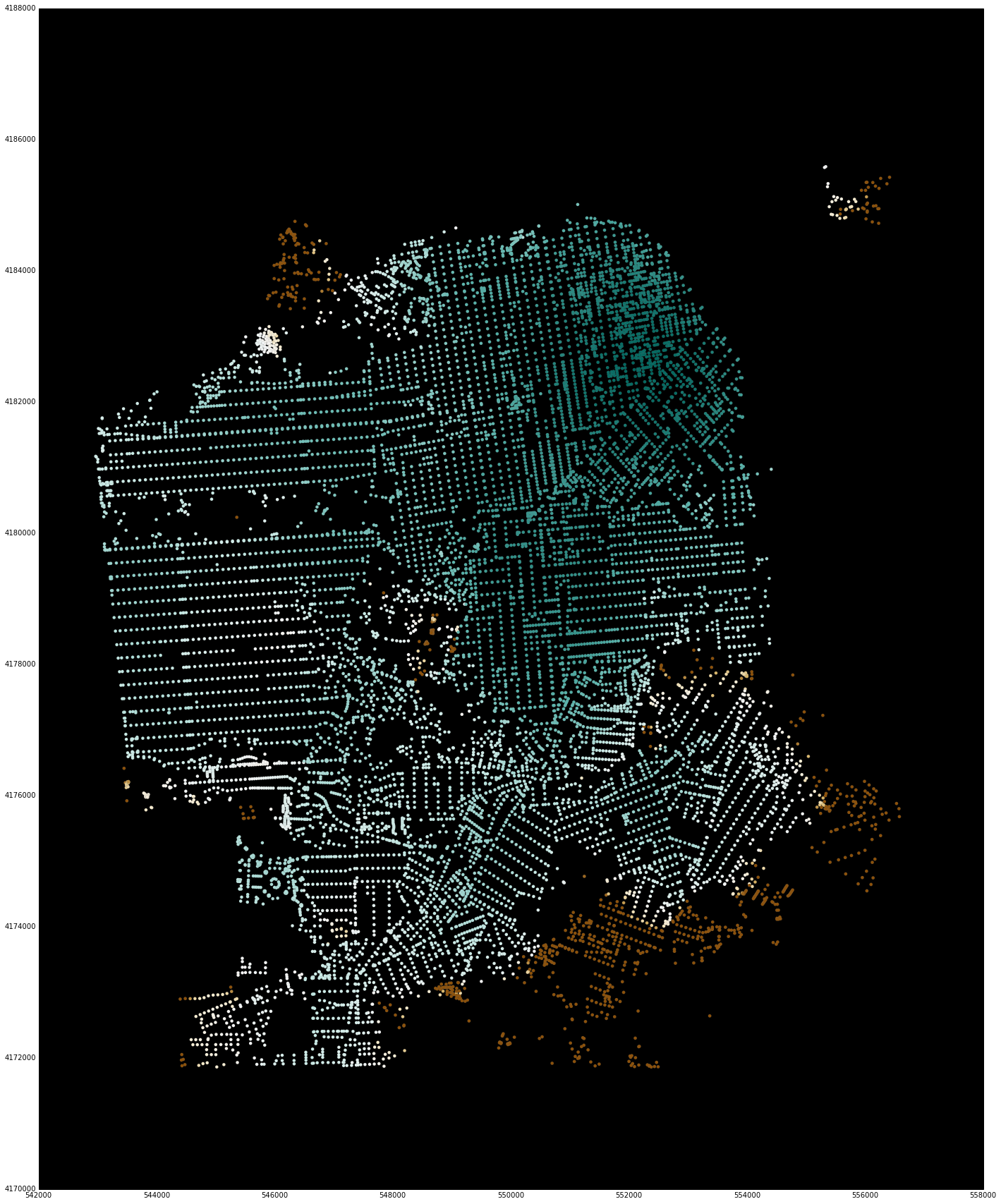
Display the results
An experimental feature for displaying the points of the node_ids and their associated computed values using matplotlib (so that the entire workflow can happen in the notebook) is also available.
Note that these have a bounding box for reducing the display window. Although the underlying library is computing values for all nodes in the region, it is difficult to visualize this much data using matplotlib. For quick interactive checking of results, the bounding box can be used to reduce the number of points that are shown, and sample code and images are included below.
sf_bbox = [37.707794, -122.524338, 37.834192, -122.34993]

net.plot(s, bbox=sf_bbox,
         fig_kwargs={'figsize': [20, 20]},
         bmap_kwargs={'suppress_ticks': False,
                      'resolution': 'h', 'epsg': '26943'},
         plot_kwargs={'cmap': 'BrBG', 's': 8, 'edgecolor': 'none'})
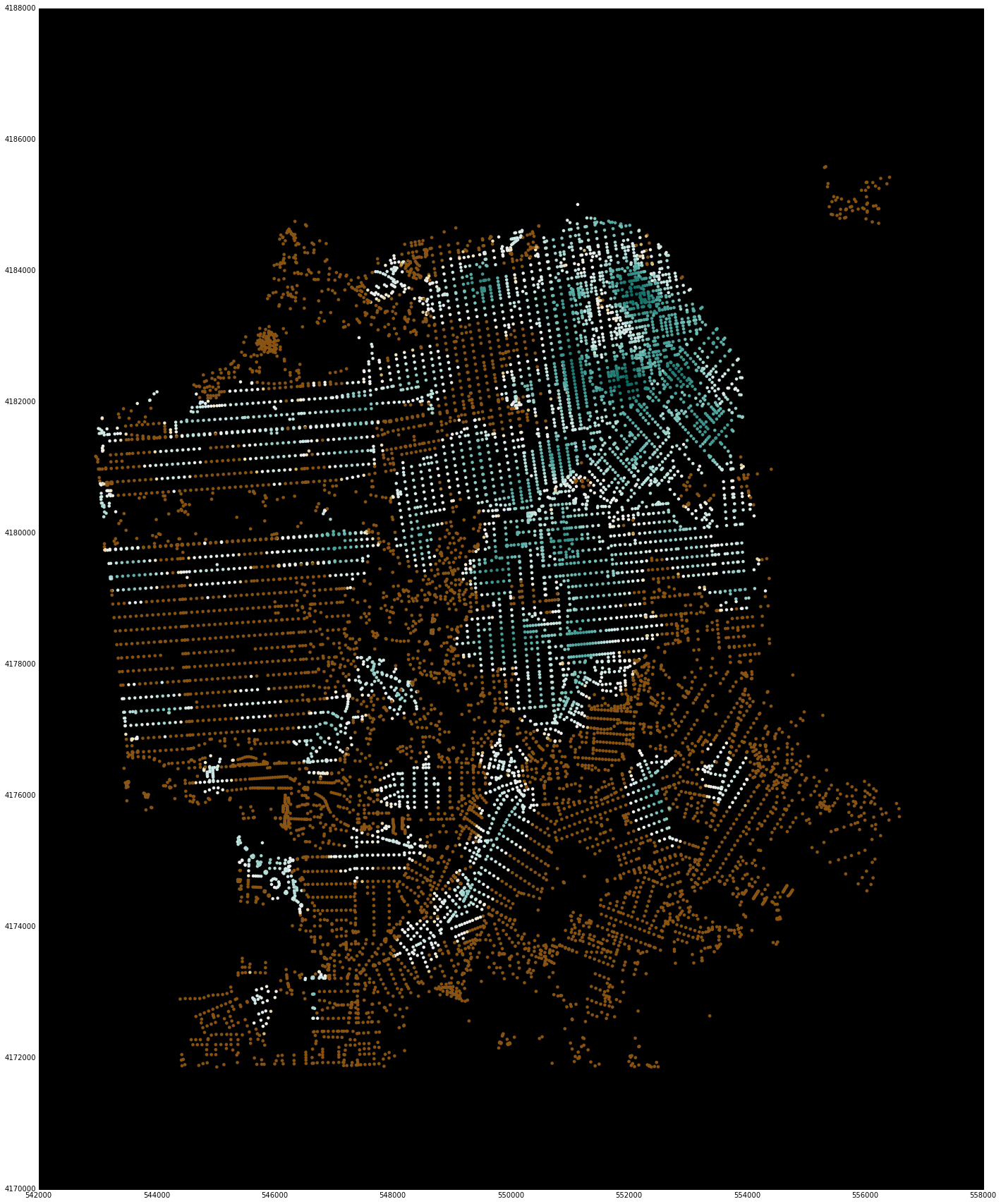
net.plot(u, bbox=sf_bbox,
         fig_kwargs={'figsize': [20, 20]},
         bmap_kwargs={'suppress_ticks': False,
                      'resolution': 'h', 'epsg': '26943'},
         plot_kwargs={'cmap': 'BrBG', 's': 8, 'edgecolor': 'none'}